Friday, September 11, 2015 – Permalink –

Locate Duplicates with Conditional Formatting

Highlight entries

Conditional formatting can be set up by selecting the whole range, or for the first cell in the range and then copy down that conditional format. I find it is usually just as easy to select the whole range to start with. The formula will adjust itself.

In this example, cell B2 has a heading of Product Numbers.

Select cell B3 (or the entire targeted range) and from the menu.

Select Format > Conditional Formatting.

The Conditional Formatting dialog opens with the initial dropdown saying
"Cell Value Is".

Click the arrow next to this, and choose
"Formula Is".

After selecting "Formula Is", the dialog box changes appearance.
Instead of boxes for "Between x and y", there is now a single formula box.

You can type in any formula as long as that formula will evaluate to TRUE or FALSE.

The formula to type in the box is
=COUNTIF(B:B,B3)>1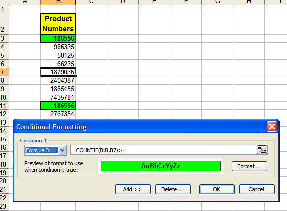



This says, "look through the entire range of column B.

Count how many cells in that range are the same value as what is in B3."
(In the graphic, B7 is the Active cell.)

That same comparison will be made in every cell that contains the conditional formatting.

(If your data is in column E and you are setting the first conditional formatting up in E5, the formula would be =COUNTIF(E:E,E5)>1.)

Anytime a duplicate appears in the range, it will receive the special formatting.

In this example, any time a duplicate number appears anywhere in column B, even if it is not itself formatted, the selected range will reflect the duplicate.

=COUNT(B:B,B3)>2 would count entries that appear more than two times.
=COUNT(B:B,B3)=2 would count entries that appear twice.

If you want only a part of the column in the formula, it is easier to use absolute addresses, such as =COUNT($B$3:$B$200,B3)>1

Adapted from MrExcel.com

Also see:
Chip Pearson's discussion of duplicates:
Duplicate And Unique Items In Lists
and:

Contextures.com:
Conditional Formatting
(See Hide Duplicate Values)


See all Topics excel

Labels: Formulas, General, Macros, Reference, Tips, Tutorials, VBA