
|
Book Home Page Bloglines 1906 CelebrateStadium 2006 OfficeZealot Scobleizer TechRepublic AskWoody SpyJournal Computers Software Microsoft Windows Excel FrontPage PowerPoint Outlook Word 

Host your Web site with PureHost! 
|
 
Sunday, January 28, 2018 – Permalink – Date ArithmaticThe drunken cousinWorking with dates has a few twists. Excel believes that time began on January 1, 1900. Each day since then is counted so that September 1, 2003 in Excel-speak would be → 37,865. 9/1/03 7:33 A.M. is a decimal → 37865.31458333333 When you subtract one date from another, for instance 9/1/2003 (A1)minus 7/4/2001 (A2), Excel displays the odd answer of → 2/27/1902. Excel formats the result of a formula with the same format as the source cells, Right-click the formula cell (=A1-A2). Select Format Cells ..., and then choose a Number format with zero decimals. The correct number of days → 789 will now be displayed. Another way is to use the rarely documented DATEDIF function. Chip Pearson calls it "the drunken cousin of the Function family." =DATEDIF(EarliestDate,LatestDate,Interval) =DATEDIF(A2,A1,"d") Here's THE source for date math: Chip Pearson: All About Dates Also: John Walenbach: Extended Date Functions Add-In "Many users are surprised to discover that Excel cannot work with dates prior to the year 1900. The Extended Date Functions add-in (XDate) corrects this deficiency, and allows you to work with dates in the years 0100 through 9999." MS Knowledge Base: How To Use Dates and Times in Excel See all Topics excel Labels: Addins, Formulas, General, Macros, Reference, Shortcuts, Tips, Tutorials <Doug Klippert@ 3:42 AM
Comments:
Post a Comment
Sunday, October 08, 2017 – Permalink – Undo ExcelLevel talkIn Excel 2007+. the number of levels of the "undo stack" was increased from 16 levels to 100. Setting AutoFilters, showing/hiding detail in PivotTables, and grouping/ungrouping in PivotTables are now reversible. And the undo stack is not cleared when Excel saves, be it an AutoSave or a Save by the user. If you think the number of undos should be changed, here's how:
 Modify the number of undo levels If you want to clear the undo stack, just run a macro such as: Sub ClearUndo()
Range("A1").Copy Range("A1")
End Sub
Allen Wyatt: Clearing the Undo stack See all Topics excel <Doug Klippert@ 3:14 AM
Comments:
Post a Comment
Friday, March 17, 2017 – Permalink – Speed up your MacroWha's a macro?"The purpose of this column is simply to provide information to anyone interested in how to make their work life more efficient through the use of macros. When your average computer user finds out that macros are all about little bits of code, the fear in their hearts becomes palpable, all the way from here. And so today I want to ease those fears and invite those of you who've been curious about macros to take the plunge and finally learn about them." Dummies.com See all Topics excel <Doug Klippert@ 3:33 AM
Comments:
Post a Comment
Saturday, November 12, 2016 – Permalink – Short Menu ChangeIn contextRight clicking an object can display a shortcut menu.Here are some instructions about how to write a macro that will edit that menu. Right Click See all Topics excel Labels: Customize, General, Macros, Reference, Shortcuts, Tips, Tutorials, VBA <Doug Klippert@ 3:55 AM
Comments:
Post a Comment
Wednesday, August 10, 2016 – Permalink – Hidden Macros Names and ShortcutsRevealedWord has built in macros to perform routine actions such as using the Format Painter to copy formatting. Rather than trying to guess the name or look up the shortcut keys, use this seldom mentioned trick to find toolbar macro names. Press the three key combination of Ctrl, Alt, and + (the plus sign on the Numbers keypad). The mouse pointer changes to a 4-leaf clover. Click on a toolbar icon. Word will display a form revealing the macro name and the assigned shortcuts. 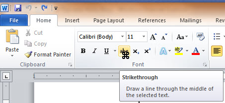 (It works the same way in 2007+) See all Topics excel <Doug Klippert@ 3:55 AM
Comments:
Post a Comment
Thursday, May 19, 2016 – Permalink – Dynamic TabsChange tab names automaticallyChanging the names of tabs is easy, just double click the tab or right click and choose rename. Allen Wyatt has a small piece of code that will automatically update the tab name based on the value of a cell in the spreadsheet. Sub myTabName()
ActiveSheet.Name = ActiveSheet.Range("A1")
End Sub
Allen also has some error checking code on his site: Dynamic Worksheet Tabs Dick Kusleika suggests another way using a change event: Naming a sheet based on a cell See all Topics excel Labels: Customize, General, Macros, Reference, Shortcuts, Tips, Tutorials, VBA <Doug Klippert@ 3:30 AM
Comments:
Post a Comment
Thursday, April 28, 2016 – Permalink – Large Text FilesSplit between worksheetsWhile this problem is alleviated in Excel 2007+ with its 1,048,576 rows by 16,348 columns, The old XL versions are still here. Text files with a large number of records are better handled in a program like Access. Having said that, there can be times that these lists must be imported into Excel. If the file has over 65,536 records, the data will not fit on a single worksheet. Here's a Microsoft Knowledge Base article with the macro code needed to bring oversized text data into Excel and split it into multiple worksheets:
Importing Text Files Larger Than 16,384/65,536 Rows Notice the code about 17 lines from the bottom of the macro. 'For xl97 and later change 16384 to 65536. Also, after import, the data must be parsed. Use Data>Text to columns. If you have not worked with macros before, Dave McRitchie has a tutorial: Getting Started with Macros and User Defined Functions See all Topics excel <Doug Klippert@ 3:28 AM
Comments:
Post a Comment
Thursday, February 18, 2016 – Permalink – Tabs with Numbers of the WeekCount to 52Excel no longer has a theoretical limit on the number of worksheets in a workbook. One common use of this ability is to add a worksheet for each week in the year. Here's a macro that does the trick: Sub YearWorkbook() Dim iWeek As Integer Dim sht As Variant Application.ScreenUpdating = False Worksheets.Add After:=Worksheets(Worksheets.Count), _ Count:=(52 - Worksheets.Count) iWeek = 1 For Each sht In Worksheets sht.Name = "Week " & Format(iWeek, "00") iWeek = iWeek + 1 Next sht Application.ScreenUpdating = True End Sub ExcelTips.VitalNews.com: Naming tabs for weeks See all Topics excel <Doug Klippert@ 3:57 AM
Comments:
Post a Comment
Thursday, December 17, 2015 – Permalink – Animate Window SizeSo cool!The following macro has little or no practical computing value, but it can add a "way cool" element when a worksheet is unhidden. There are three states that a worksheet can be in; Minimized, Maximized, and Normal. From AutomateExcel.com: ActiveWindow.WindowState (By Mark William Wielgus) Also fun: Sub SheetGrow() Dim x As Integer, xmax As Integer With ActiveWindow .WindowState = xlNormal .Top = 1 .Left = 1 .Height = 50 .Width = 50 If Application.UsableHeight > Application.UsableWidth Then xmax = Application.UsableHeight Else xmax = Application.UsableWidth End If For x = 50 To xmax If x <= Application.UsableHeight Then .Height = x If x <= Application.UsableWidth Then .Width = x Next x .WindowState = xlMaximized End With End Sub # posted by Joerd See all Topics excel Labels: Customize, General, Macros, Reference, Tips, Tutorials, VBA <Doug Klippert@ 3:45 AM
Comments:
Post a Comment
Friday, September 25, 2015 – Permalink – Time Without LimitsNo DelimitersExcel is most happy when you enter dates and times with the correct separators. 1/1/2004 is a good date. So is 1-1-2004. If you just entered 112004 in a cell formatted as a date you'll get: Wednesday, August 27, 2206 the 112,004th day since January 1, 1900. Chip Pearson has come up with VBA code, using the Worksheet_Change event procedure, that will allow you to enter dates without dashes or slashes.  See: Date And Time Entry See all Topics excel Labels: Formats, Functions, Macros, Reference, Shortcuts, Tips, Tutorials, VBA <Doug Klippert@ 3:55 AM
Comments:
Post a Comment
Friday, September 11, 2015 – Permalink – Locate Duplicates with Conditional FormattingHighlight entriesConditional formatting can be set up by selecting the whole range, or for the first cell in the range and then copy down that conditional format. I find it is usually just as easy to select the whole range to start with. The formula will adjust itself. In this example, cell B2 has a heading of Product Numbers. Select cell B3 (or the entire targeted range) and from the menu. Select Format > Conditional Formatting. The Conditional Formatting dialog opens with the initial dropdown saying "Cell Value Is". Click the arrow next to this, and choose "Formula Is". After selecting "Formula Is", the dialog box changes appearance. Instead of boxes for "Between x and y", there is now a single formula box. You can type in any formula as long as that formula will evaluate to TRUE or FALSE. The formula to type in the box is =COUNTIF(B:B,B3)>1 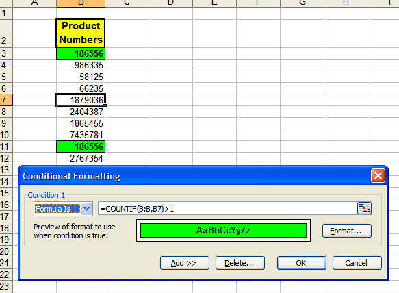 This says, "look through the entire range of column B. Count how many cells in that range are the same value as what is in B3." (In the graphic, B7 is the Active cell.) That same comparison will be made in every cell that contains the conditional formatting. (If your data is in column E and you are setting the first conditional formatting up in E5, the formula would be =COUNTIF(E:E,E5)>1.) Anytime a duplicate appears in the range, it will receive the special formatting. In this example, any time a duplicate number appears anywhere in column B, even if it is not itself formatted, the selected range will reflect the duplicate. =COUNT(B:B,B3)>2 would count entries that appear more than two times. =COUNT(B:B,B3)=2 would count entries that appear twice. If you want only a part of the column in the formula, it is easier to use absolute addresses, such as =COUNT($B$3:$B$200,B3)>1 Adapted from MrExcel.com Also see: Chip Pearson's discussion of duplicates: Duplicate And Unique Items In Lists and: Contextures.com: Conditional Formatting (See Hide Duplicate Values) See all Topics excel Labels: Formulas, General, Macros, Reference, Tips, Tutorials, VBA <Doug Klippert@ 3:11 AM
Comments:
Post a Comment
Thursday, September 10, 2015 – Permalink – Sort worksheetsOrder tabsWorksheets can be dragged and dropped into any order required. They can be set up in numeric or alpha order, but doing it by hand is a bother. Chip Pearson has written some macros that will do the job for you:
Here's the code to sort by tab color: Sub GroupSheetsByColor() Sorting Worksheets In A Workbook (The colorindex variable chooses one of the 56 colors in Excel's basic palette. Here are all the colors and numbers as compiled by F. David McRitchie:Excel Colors ) See all Topics excel <Doug Klippert@ 3:26 AM
Comments:
Post a Comment
Friday, August 14, 2015 – Permalink – CalendarOne day at a timeHere are some links with downloadable examples, and some code that can be used to create calendars in Excel: Andrew Engwirda's Excel tips: Excel Calendar Calendar Toolbar He also suggests: "Tushar Mehta has a very nice calendar too which can be found here: Erlandsen Data Consulting: "Create a Create a simple calendar for each month or a small calendar (pocket) for a whole year. MakeCalendarPlanner() (Evelyn Woolston scroll down to entry #5) Microsoft Templates: Calendar templates See all Topics excel Labels: General, Macros, Reference, Templates, Tips, Tutorials, VBA <Doug Klippert@ 3:29 AM
Comments:
Post a Comment
Tuesday, July 21, 2015 – Permalink – List All FilesAll files in a folderHere is a macro that will produce a list of all the files in a selected folder.
 Macro to List All Files in a Folder Macro to List All Files in a Folder
See all Topics excel <Doug Klippert@ 3:41 AM
Comments:
Post a Comment
Saturday, June 06, 2015 – Permalink – Formatting Code for Headers and FootersRoll your ownFrom Microsoft support: The following list contains the format codes that you can use in headers and footers. Codes to format text ("&" is an ampersand - Shift+7) &L (font. Be sure to include the quotation marks around the font name.) (font size. Use a two-digit number to specify a size in points.) Codes to insert specific data &D
In a macro, to use multiple lines in a header, use either of the following methods:
Microsoft KB213618 Also: Daily Dose of Excel: Formatting Footers in VBA See all Topics excel Labels: Formats, General, Macros, Reference, Shortcuts, Tips, Tutorials, VBA <Doug Klippert@ 3:42 AM
Comments:
Post a Comment
Thursday, May 28, 2015 – Permalink – Run a Macro From a CellHow to do the impossible (almost)There are times when it might be nice to run a macro from a cell function. Something like : if a cell has a certain value, a macro will run: =IF(A1>10,Macro1) You can not initiate a macro from a worksheet cell function. However, you can use the worksheet's Change event to do something like this: When A1 is changed to a value greater than 10, the macro code will run. To get to the Worksheet Event code, right-click the sheet tab and choose View Code.  From CPearson.com Also see: Change Events Also: Microsoft KnowledgeBase: How to Run a Macro When Certain Cells Change After posting this, Ross Mclean came up with a great work around using a User Defined Function. Keep in mind that some commands will be ignored. A macro run from the worksheet like this will not change the Excel environment. For example (watch line wrap), this VBA code: Public Function RMAC _ (ByVal Macro_Name As String, _ ByVal Arg1 As Variant) RMAC = Application.Run _ (Macro_Name, Arg1) End Function Sub MyMacro(arg As String) ActiveCell.Interior.ColorIndex _ = 3 Beep End Sub when invoked by this worksheet formula: =rmac("MyMacro","yada")
runs the sub MyMacro with some modification. The Beep is executed, the cell color change is not. - Jon ------- Jon Peltier, Microsoft Excel MVP Peltier Technical Services Tutorials and Custom Solutions http://PeltierTech.com/ See all Topics excel <Doug Klippert@ 3:47 AM
Comments:
Post a Comment
Wednesday, May 27, 2015 – Permalink – Signing MacrosSecurity levelsThere are three levels of Macro security:
"If you've used Access 2003, you've probably seen several security warning messages - Access 2003 cares about your security. An important part of Access 2003 security is digitally signing your code. As Rick Dobson shows, you can do it, but preparing for digital signing is critical.Also: Signing Access Projects Other links: How to make sure that your Office document has a valid digital signature in 2007 Office products and in Office 2003 See all Topics excel <Doug Klippert@ 3:14 AM
Comments:
Post a Comment
Thursday, May 14, 2015 – Permalink – Show Formulas in Cell CommentsDisplay propertiesSelect the cells and then run this macro: 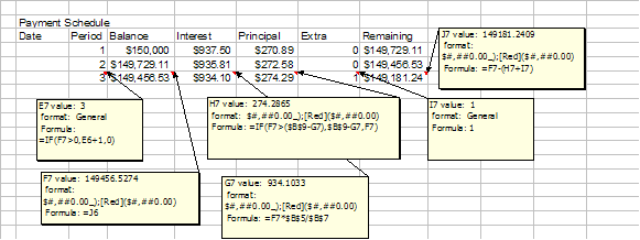 by David McRitchie Also: Show FORMULA of another cell in Excel See all Topics excel Labels: Formulas, General, Macros, Reference, Tips, Tutorials, VBA <Doug Klippert@ 3:37 AM
Comments:
Post a Comment
Sunday, May 10, 2015 – Permalink – Customize date in footerFormattingThis subroutine inserts the current date in the footer of all sheets in the active workbook. This process can be accomplished without a macro, however, you'll need the macro if you want to specify the formatting of the current date. An example of the return generated by running this macro is Saturday, May 10, 2015. You can change the word CenterFooter to CenterHeader. You could also use LeftHeader, RightHeader, LeftFooter, or RightFooter. Microsoft KnowledgeBase: Macro to Change the Date/Time Format in a Header/Footer See all Topics excel Labels: Customize, Formats, General, Macros, Reference, Tips, Tutorials, VBA <Doug Klippert@ 3:48 AM
Comments:
Post a Comment
Wednesday, April 29, 2015 – Permalink – PrintingMacro controlHere are some useful macros concerning Excel and printing. They were written by Ole P. Erlandsen of: ERLANDSEN DATA CONSULTING
See all Topics excel Labels: Customize, Formats, General, Macros, Reference, Shortcuts, Tips, Tutorials, VBA <Doug Klippert@ 3:28 AM
Comments:
Post a Comment
|
