Unofficial Excel Stuff

Book

Suggestions

Home Page

Bloglines

1906
CelebrateStadium
2006

OfficeZealot

Scobleizer

TechRepublic

AskWoody

SpyJournal

Wednesday, December 27, 2017 – Permalink –

All the Basics

All(most) all you need to know

Office.Microsoft.com has a short demo that shows you the main things anyone needs to know about Excel.

There are many thousands of users who find that this is all they ever need.

Add numbers

Subtract numbers

Multiply numbers

Divide numbers

Use simple formulas to do the math

See all Topics excel
Labels: Formulas, Functions, General, Reference, Tips, Tutorials

<Doug Klippert@ 3:45 AM

Comments: Post a Comment

Tuesday, December 19, 2017 – Permalink –

Loan Payment

Basic tutorial

Microsoft provides a number of learning activities related to fundamental tasks.

Here's one that walks the student through a worksheet designed to calculate interest and total payment for a purchase, based on different loan terms.

"This practical spreadsheet lesson offers easy answers to life's perplexing math problems like How much will my dream car really cost after financing?

Students will calculate the cost of purchasing their very own Lamborghini sports car and determine if the ultimate price tag is really worth the investment. "

Dream Car
Also:
Basic Financial Calculations

See all Topics excel
Labels: Formulas, Functions, General, Reference, Shortcuts, Templates, Tips, Tutorials

<Doug Klippert@ 3:23 AM

Comments: Post a Comment

Tuesday, October 31, 2017 – Permalink –

Calculate Running Total

Using the OFFSET function

Adding up a running balance can be frustrating when new data is added or old transactions are removed.

"How to create a data list to manage transactions, add and delete rows from the list, and accurately calculate a running balance using the OFFSET function."
Cash flow using OFFSET.PDF

Office.Microsoft.com:
Calculate a running total

See all Topics excel
Labels: Formulas, Functions, General, Reference, Shortcuts, Tips, Tutorials

<Doug Klippert@ 3:13 AM

Comments: Post a Comment

Thursday, October 26, 2017 – Permalink –

Insert Line Breaks With Code

Label Captions

If you've ever needed to insert line breaks in a message box prompt, you most likely built a string that incorporated a line feed or carriage return character. Unfortunately, label objects aren't as forgiving when it comes to using these characters.

If you're setting a label's Caption property with code, you'll find that the special control characters are interpreted as squares, since they're otherwise un-displayable.
To successfully insert a line break in a label caption, you need to include both a line feed character and a carriage return character, entered consecutively.

To do so, you can use the Chr() function, such as:

Me.Label1.Caption = "Line 1" & _ Chr(13) & Chr(10) & "Line 2"

However, you can also simplify your code using an built-in constant:

Me.Label1.Caption = "Line 1" & vbCrLf & "Line 2"

See all Topics excel
Labels: Formats, Functions, General, Reference, Shortcuts, Tips, Tutorials

<Doug Klippert@ 3:08 AM

Comments: Post a Comment

Thursday, August 31, 2017 – Permalink –

Tips and Formulae

Functions and Macros

I'm always looking for Excel sites. A fresh perspective can make the view more clear.
While he does approach from a Mac angle, the Excel world welcomes those of all persuasions.

J.E. McGimpsey's XL Pages

Here are some of the tips:

Remove internal worksheet/workbook protection

Why your sum is a penny off...

Highlight row without losing color formatting

Why use -- in SUMPRODUCT formulae

Using SUMPRODUCT() to calculate variable rates and commissions

Three-dimensional SUMIF()s

Bitwise Logical Functions

Sampling from a range

Summing every Nth column or row

Worksheet and Workbook names using the CELL() function

See all Topics excel
Labels: Formulas, Functions, General, Reference, Shortcuts, Tips, Tutorials

<Doug Klippert@ 3:15 AM

Comments: Post a Comment

Monday, May 08, 2017 – Permalink –

Statistical Functions

Definitions and list

Excel contains a slew of functions relating to statistical analysis.

That's a slew not a skew.

SKEW(number1,number2,...)

Returns the skewness of a distribution. Skewness characterizes the degree of asymmetry of a distribution around its mean.

Positive skewness indicates a distribution with an asymmetric tail extending toward more positive values.

Negative skewness indicates a distribution with an asymmetric tail extending toward more negative values.

Statistical Functions

Training - Statistical

See all Topics excel
Labels: Functions, General, Reference, Tips, Tutorials

<Doug Klippert@ 3:51 AM

Comments: Post a Comment

Tuesday, January 24, 2017 – Permalink –

Custom Functions

Write your own
Excel allows you to create your own functions. If =SUM() is not enough for you, look at this link:

Custom Functions - User Defined Functions

See all Topics excel
Labels: Customize, Functions, General, Reference, Tips, Tutorials

<Doug Klippert@ 3:10 AM

Comments: Post a Comment

Monday, August 15, 2016 – Permalink –

Display Row, Column Headings

User Function

Here's an odd little use of functions.

If you want to display the Row number on a spreadsheet, the formula

=Row()
works just fine.
You could then hide the Row and Column headings and format the Row numbers any way you want. If a Row is deleted the numbers will automatically update.

Column headings are a little harder. The formula =Column() will show the number of the Column, not the letter, i.e. "2" instead of "B".

The following formula extracts the Column letter:

=SUBSTITUTE(ADDRESS(1,COLUMN(),4),"1","")

To break it down:

=ADDRESS(row_num,column_num,abs_num)

This finds the address at Row number "1" and current Column number. The abs_num of "4 " says make the result a relative address.

The formula will produce a result such as "AA1".

SUBSTITUTE(text,old_text,new_text)

This function looks at the address, i.e. "AA1".
It replaces the Row number character ("1") with a null or empty value ("").
The formula will produce a result such as "AA".

Also see Daily Dose of Excel by Dick Kusleika.

Dick mused:'

"Sometime before the year 3,000, Microsoft will hopefully increase the number of columns in Excel (Hey, I can dream can't I). The challenge before you is to write a function that converts a column number to its letter equivalent assuming columns go to ZZZZ. That’s about 450,000 columns - maybe more than I need."

Of course Office 2007+ has taken it up to 16,284 columns.

See all Topics excel
Labels: Functions, General, Reference, Shortcuts, Tips, Tutorials, VBA

<Doug Klippert@ 3:27 AM

Comments: Post a Comment

Saturday, June 11, 2016 – Permalink –

When 28 is 30

How long is a month?

When you use the banker's DAYS360 function to calculate the number of days between two dates, you can get an odd answer.

If you use the DAYS360 function with a start date of February 28 and with an end date of March 28, a value of 28 days is returned.
You expect a value of 30 days to be returned for every full month. (12*30=360)

This behavior may occur if you use the U.S. method, also known as the NASD method, with the DAYS360 function.

To work around this behavior, use the European method with the DAYS360 function. With the European method starting dates and ending dates that occur on the 31st of a month become equal to the 30th of the same month. To use the European method with the DAYS360 function, use the following syntax:

=DAYS360(cell number of start date,cell number of end date,TRUE)

Using FALSE or omitting the third parameter uses the U.S. method

Support.microsoft.com
An unexpected value with the DAYS360 function

See all Topics excel
Labels: Functions, General, Reference, Tips, Tutorials, VBA

<Doug Klippert@ 3:43 AM

Comments: Post a Comment

Saturday, May 28, 2016 – Permalink –

Declaring Multiple Variables

Declare each one

When setting up a macro in VBA, if you want to declare multiple variables in one line of code, be sure to specify the type for each variable, even if the variables are the same type. Avoid code like the following:

Dim strFName, strLName, strMI As String

In such a case, only the last variable, strMI, is actually declared as a String type. The first two variables are designated by default as Variant data types.

To correctly declare the three variables, you would use the statement:

Dim strFName As String, strLName As String, strMI As String

See all Topics excel
Labels: Functions, General, Reference, Tips, Tutorials

<Doug Klippert@ 3:49 AM

Comments: Post a Comment

Sunday, March 06, 2016 – Permalink –

Count the Colors

I bid 3 Red

What if you would like to know the color name or to count or to sum cells by a fill color? There is no built-in function in Excel.

In this case you can make a User Defined Function (UDF).

Here is the sample UDF that you can use to analyze, count and sum the cells depending on their filled color.

These UDF function can be used in the same way as built-in functions that you can use in the worksheet.

AnalyzeColor Returns the color name, the color index or color index in RGB.
Syntax: AnalyzeColor(color range, optional; "text" or "index" or "rgb". When it is omitted "text" is used.)

CountColor Counts the number of cells depending on their filled color.
Syntax: CountColor(color range, target range)

SumColor Adds all the numbers in a range of cells depending on their filled color.
Syntax: SumColor(color range, target range)

Sum and Count by fill color

Chip Pearson:
Working with Cell Colors

See all Topics excel
Labels: Formulas, Functions, Reference, Tips, Tutorials, VBA

<Doug Klippert@ 3:37 AM

Comments: Post a Comment

Monday, February 22, 2016 – Permalink –

UDF is not a Baby Alien

Things should to function

Frank Rice has written a "show how" about creating functions that are not included in the box.

"Excel allows you to create custom functions, called "User Defined Functions" (UDF's) that can be used the same way you would use SUM(), VLOOKUP, or other built-in Excel functions.
The Excel user who wishes to use advanced mathematics or perform text manipulation is often seriously disappointed by Excel's limited library of formulas and functions. A UDF is simply a function that you create yourself with VBA.

The following is a sample that is a good candidate for a UDF:

Function CtoF(Centigrade) CtoF = Centigrade * 9 / 5 + 32 End Function

In the Worksheet you would enter something like:
=CtoF(A1)
frice's Weblog

Here are some other links:

Vertex42.com:
User Defined Functions

Support.Microsoft.com:
Functions to Calculate Light Years

See all Topics excel
Labels: Formulas, Functions, General, Reference, Tips, Tutorials

<Doug Klippert@ 3:46 AM

Comments: Post a Comment

Friday, January 29, 2016 – Permalink –

Lookup, Down, and Sideways

A very useful Excel feature

Excel does not have "relational" tables like database applications such as Access.

You, however, can make use of database functions including the ability to look up values in a table based on a value.

You could, for instance look up a salesperson's records based on an employee ID.

Using VLOOKUP, HLOOKUP, INDEX, and MATCH in Excel to interrogate data tables

John Walkenbach has a book "Excel 2003 Formulas" with a 24-page chapter on Lookup functions and other database/list tricks.

Chip Pearson talks about lookups on his site as well..

Daily Dose of Excel:
VLookup on Two Comumns

See all Topics excel
Labels: Formulas, Functions, General, Reference, Tips, Tutorials

<Doug Klippert@ 3:49 AM

Comments: Post a Comment

Friday, September 25, 2015 – Permalink –

Time Without Limits

No Delimiters

Excel is most happy when you enter dates and times with the correct separators.

1/1/2004 is a good date. So is 1-1-2004.

If you just entered 112004 in a cell formatted as a date you'll get:

Wednesday, August 27, 2206

the 112,004^th day since January 1, 1900.

Chip Pearson has come up with VBA code, using the Worksheet_Change event procedure, that will allow you to enter dates without dashes or slashes.

See:
Date And Time Entry

See all Topics excel
Labels: Formats, Functions, Macros, Reference, Shortcuts, Tips, Tutorials, VBA

<Doug Klippert@ 3:55 AM

Comments: Post a Comment

Sunday, September 20, 2015 – Permalink –

Information Functions

Who, What, Where

If you need to know if automatic calculation is on or off or the number of worksheets that are active, Excel can display the INFO.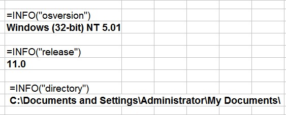

System Information:

Current directory

=INFO("directory")

Available bytes of memory

=INFO("memavail")

Memory in use

=INFO("memused")

Total bytes of memory

=INFO("totmem")

Number of active worksheets

=INFO("numfile")

Cell currently in the top left of the window

=INFO("origin")

Operating system

=INFO("osversion")

Recalculation mode

=INFO("recalc")

Excel version

=INFO("release")

Name of system. (PC or Mac)

=INFO("system")

See all Topics
Labels: Functions, General, Reference, Tips

<Doug Klippert@ 3:42 AM

Comments: Post a Comment

Friday, August 07, 2015 – Permalink –

Stock Answer

Built in service

You can easily insert an automatically updated stock quote for a specific company in a spreadsheet.

Here are the instructions:

On the Tools menu, click AutoCorrect options.
(Use the Office button and Excel Options in 2007+)

Click the Smart Tags tab and place a check beside Label data with smart tags.

Click OK.

Type in a Stock symbol (such as MSFT) in a cell.
(The symbol must be in all caps)

Click outside of the cell.

Place your mouse cursor over the purple triangle in the lower-right corner of the cell.
Click the arrow.

Click Insert refreshable stock price.

Select whether to insert the stock price on a new worksheet or in a specific area on your current worksheet.

You can refresh a stock quote price at any time by right clicking anywhere within your worksheet and selecting Data Range Properties. Enter a value for how often the stock quote price should be refreshed.

See all Topics
Labels: Functions, General, Reference, Shortcuts, Tips, Tutorials

<Doug Klippert@ 3:20 AM

Comments: Post a Comment

Wednesday, July 22, 2015 – Permalink –

Statistics and Excel

What are the chances

"Excel is the widely used statistical package, which serves as a tool to understand statistical concepts and computation to check your hand-worked calculation in solving your homework problems. The site provides an introduction to understand the basics of and working with the Excel. Redoing the illustrated numerical examples in this site will help improving your familiarity and as a result increase the effectiveness and efficiency of your process in statistics."

Dr. Hossein Arsham

The site is very clearly written. While some of the concepts are advanced, Dr. Arsham explains them in simple terms. It is a good introduction to the Analysis ToolPak.

Here are some of the subjects covered:

Descriptive Statistics

Normal Distribution

Confidence Interval for the Mean

Test of Hypothesis Concerning the Population Mean

Difference Between Mean of Two Populations

ANOVA: Analysis of Variances

Goodness-of-Fit Test for Discrete Random Variables

Test of Independence: Contingency Tables

Test Hypothesis Concerning the Variance of Two Populations

Linear Correlation and Regression Analysis

Moving Average and Exponential Smoothing

The University of Baltimore: Statistical Data Analysis

See all Topics excel
Labels: Formulas, Functions, General, Reference, Tips, Tutorials

<Doug Klippert@ 3:11 AM

Comments: Post a Comment

Saturday, May 30, 2015 – Permalink –

Date Calculations

Day by Day
How to count the days. Definitions and equations.

Date Calculations in Excel

by Charley Kyd

See all Topics excel
Labels: Formulas, Functions, General, Reference, Tips, Tutorials, VBA

<Doug Klippert@ 3:54 AM

Comments: Post a Comment

Saturday, May 23, 2015 – Permalink –

Column(s) Function

VLOOKUP

"Excel will adjust cell references in formulas when you insert or delete rows or columns.

For example, if the cell C1 contains the formula =A1/B1 and you insert a column to the left of column A; the formula will change to =A1/C1.

The problem then occurs with VLOOKUP. Its column index number argument is a simple number, not a reference.

VLOOKUP(lookup_value,table_array,col_index_num,range_lookup

For Example:

Choose a blank worksheet

In cells A1 and A2, enter the values 1 and 2.

In B1 and B2, enter Jan and Feb.

Select all four cells and drag the fill handle at the bottom right-hand corner of the selection downward to row 12.

You should now have the numbers 1 through 12 in column A and the months Jan through Dec in column B. In cell D1 enter the formula =VLOOKUP(C1,A1:B12,2). Now enter any number from 1 to 12 in cell C1. The formula will select the corresponding month name. To demonstrate the problem, right-click on the heading of column B and choose Insert. The formula changes to =VLOOKUP (D1,A1:C12,2), which returns 0. Excel correctly changed the cell reference from C1 to D1 and expanded the lookup range to include the inserted column, but it cannot change the column index number. Press Ctrl-Z to undo the column insertion. The solution is to modify the formula so that the column index number is not hard-coded but instead is calculated from cell references. You could use the COLUMN() function that returns the column number of the reference and, as in this example, compute the number of columns between the first and last columns: =VLOOKUP (C1,A1:B12,COLUMN(B1)-COLUMN(A1)+1). A more esthetically pleasing, or sophisticated, function might be: COLUMNS(array) This returns the number of columns in an array or reference. The modified lookup function looks like this: =VLOOKUP (C1,A1:B12,COLUMNS(A1:B1)). Either way, now if a column is inserted in the middle of the range, the column index will be adjusted."
From a PC Magazine article By Neil J. Rubenking

Also: eHow: Using the Column Function

OzGrid: Copy Rows (Scroll down to about the middle of the page)

See all Topics excel
Labels: Functions, General, Reference, Tips, Tutorials

<Doug Klippert@ 3:27 AM

Comments: Post a Comment