
|
Book Home Page Bloglines 1906 CelebrateStadium 2006 OfficeZealot Scobleizer TechRepublic AskWoody SpyJournal Computers Software Microsoft Windows Excel FrontPage PowerPoint Outlook Word 

Host your Web site with PureHost! 
|
 
Friday, April 20, 2018 – Permalink – Week NumbersWho's counting?For most purposes, weeks are numbered with Sunday considered the first day of the week. This works most of the time, but it can be a little confusing certain years. 2004 had 53 weeks. January 1 is the only day in the first week of 2005. Week 2 starts on Sunday 1/2/2005. Chip Pearson is the Date and Time guy: Week Numbers In Excel "Under the International Organization for Standardization (ISO) standard 8601, a week always begins on a Monday, and ends on a Sunday. The first week of a year is that week which contains the first Thursday of the year, or, equivalently, contains Jan-4. The first week of 2005 should start on January 3. The first and second would be part of week 53 of 2004. Wikipedia: Week Dates If your week starts on a different day, you can use the Analysis ToolPac function: =WEEKNUM(A1, 2) for a week that starts on Monday, =WEEKNUM(A1) if it starts on Sunday. Also this from ExcelTip.com: Weeknumbers using VBA in Microsoft Excel "The function WEEKNUM() in the Analysis Toolpack addin calculates the correct week number for a given date, if you are in the U.S. The user defined function shown here will calculate the correct week number depending on the national language settings on your computer." In Access: DatePart Function If your work week is always Saturday through Friday then datepart("ww",[DateField],7,1) will return 1 for 1/1/2005 through 1/7/2005, 2 for January 8-14/2005, etc. Otherwise use 1 for Sunday through 7 for Saturday. The last number sets these parameters: 1, Start with week in which January 1 occurs (default). 2, Start with the first week that has at least four days in the new year. 3, Start with first full week of the year. See all Topics excel Labels: Formulas, General, Reference, Shortcuts, Tips, Tutorials <Doug Klippert@ 3:25 AM
Comments:
Post a Comment
Sunday, January 28, 2018 – Permalink – Date ArithmaticThe drunken cousinWorking with dates has a few twists. Excel believes that time began on January 1, 1900. Each day since then is counted so that September 1, 2003 in Excel-speak would be → 37,865. 9/1/03 7:33 A.M. is a decimal → 37865.31458333333 When you subtract one date from another, for instance 9/1/2003 (A1)minus 7/4/2001 (A2), Excel displays the odd answer of → 2/27/1902. Excel formats the result of a formula with the same format as the source cells, Right-click the formula cell (=A1-A2). Select Format Cells ..., and then choose a Number format with zero decimals. The correct number of days → 789 will now be displayed. Another way is to use the rarely documented DATEDIF function. Chip Pearson calls it "the drunken cousin of the Function family." =DATEDIF(EarliestDate,LatestDate,Interval) =DATEDIF(A2,A1,"d") Here's THE source for date math: Chip Pearson: All About Dates Also: John Walenbach: Extended Date Functions Add-In "Many users are surprised to discover that Excel cannot work with dates prior to the year 1900. The Extended Date Functions add-in (XDate) corrects this deficiency, and allows you to work with dates in the years 0100 through 9999." MS Knowledge Base: How To Use Dates and Times in Excel See all Topics excel Labels: Addins, Formulas, General, Macros, Reference, Shortcuts, Tips, Tutorials <Doug Klippert@ 3:42 AM
Comments:
Post a Comment
Wednesday, December 27, 2017 – Permalink – All the BasicsAll(most) all you need to knowOffice.Microsoft.com has a short demo that shows you the main things anyone needs to know about Excel. There are many thousands of users who find that this is all they ever need.
See all Topics excel Labels: Formulas, Functions, General, Reference, Tips, Tutorials <Doug Klippert@ 3:45 AM
Comments:
Post a Comment
Tuesday, December 19, 2017 – Permalink – Loan PaymentBasic tutorialMicrosoft provides a number of learning activities related to fundamental tasks. Here's one that walks the student through a worksheet designed to calculate interest and total payment for a purchase, based on different loan terms. "This practical spreadsheet lesson offers easy answers to life's perplexing math problems like How much will my dream car really cost after financing? Dream Car Also: Basic Financial Calculations See all Topics excel Labels: Formulas, Functions, General, Reference, Shortcuts, Templates, Tips, Tutorials <Doug Klippert@ 3:23 AM
Comments:
Post a Comment
Tuesday, October 31, 2017 – Permalink – Calculate Running TotalUsing the OFFSET functionAdding up a running balance can be frustrating when new data is added or old transactions are removed. "How to create a data list to manage transactions, add and delete rows from the list, and accurately calculate a running balance using the OFFSET function."Cash flow using OFFSET.PDF Office.Microsoft.com: Calculate a running total See all Topics excel Labels: Formulas, Functions, General, Reference, Shortcuts, Tips, Tutorials <Doug Klippert@ 3:13 AM
Comments:
Post a Comment
Thursday, August 31, 2017 – Permalink – Tips and FormulaeFunctions and MacrosI'm always looking for Excel sites. A fresh perspective can make the view more clear. While he does approach from a Mac angle, the Excel world welcomes those of all persuasions. J.E. McGimpsey's XL Pages Here are some of the tips:
See all Topics excel Labels: Formulas, Functions, General, Reference, Shortcuts, Tips, Tutorials <Doug Klippert@ 3:15 AM
Comments:
Post a Comment
Wednesday, August 23, 2017 – Permalink – Location IndicatorPoint to the spotHere's a link to the code that produces conditional formatting on the fly to the cells in the current row and column.  Color banding location See all Topics excel Labels: Formats, Formulas, General, Reference, Tips, Tutorials <Doug Klippert@ 3:33 AM
Comments:
Post a Comment
Wednesday, July 26, 2017 – Permalink – Hide DupsFormat don't showDuplicate entries can be formatted to "disappear", but still be available for computation.
Also: Hide Records with Duplicate Cell Entries See all Topics excel Labels: Formulas, General, Reference, Shortcuts, Tips, Tutorials <Doug Klippert@ 3:17 AM
Comments:
Post a Comment
Tuesday, May 02, 2017 – Permalink – Result is a pictureIf 4, show kumquatAllen Wyatt has a cool procedure that will let you show a picture of an object on your spreadsheet depending on a value. Maybe a snow suit when it's 29 or, say, a pair of bloomers when the computed temperature is 70. The procedure does not use any VBA, just equations and bright thinking. ExcelRibbon.Tips.net Display Images based on a Result See all Topics excel Labels: Customize, Formulas, General, Graphics, Reference, Shortcuts, Tips, Tutorials <Doug Klippert@ 3:55 AM
Comments:
Post a Comment
Sunday, April 23, 2017 – Permalink – Worksheet NameFormula constructionThere may come a time when you need to display the name of a worksheet. This formula will do the job: =MID(CELL("filename",$A$1),FIND("]",CELL("filename",$A$1))+1,31)
=CELL("filename",$A$1)
returns the path, the Workbook name and the Worksheet name. (C:\Documents\[April.xls]\Costs)=MID(text,start_num,num_chars)selects the text that starts at a certain point and goes on for a certain number of characters. The formula, as written, looks at the full path and selects the first time a closing bracket (]) is found. It then moves 1 character to the right and displays the results up to 31 characters. (A worksheet name cannot be more that 31 characters long.) You could include a reference to that cell on other worksheets. See all Topics excel <Doug Klippert@ 3:56 AM
Comments:
Post a Comment
Saturday, November 19, 2016 – Permalink – Sparklines 2013Hail TufteNew for Excel 2010-13See all Topics excel Labels: Charts, Formats, Formulas, General, Reference, Tips, Tutorials <Doug Klippert@ 8:22 AM
Comments:
Post a Comment
Tuesday, August 09, 2016 – Permalink – Curvesand More Here is a collection of Functions relating to astronomy from Stargazing.net. Can't tell who might be interested in the obliquity of the equator given date in days after J2000.0. See: Astro VBA Other Curve stuff: DelphiForFun.org: converting polar coordinates to Cartesian coordinates. "Students of analytic geometry, (the kind that combines algebra and geometry), often work in one of two coordinate systems: Cartesian or Polar - and frequently must convert from one to the other. See all Topics excel Labels: Charts, Formulas, General, Reference, Tips, Tutorials <Doug Klippert@ 3:58 AM
Comments:
Post a Comment
Tuesday, March 29, 2016 – Permalink – Thirtieth Condition FormattingThree is not always enoughPre-2007 Excel gives the user the ability to specify up to three conditions under Format>Conditional Formatting. If that is not enough, here's the code that extends the conditions to 30!  Extended Conditional Formatter Also see: Conditional Formatting (including 2007) See all Topics excel Labels: Customize, Formats, Formulas, General, Reference, Shortcuts, Tips, Tutorials, VBA <Doug Klippert@ 3:09 AM
Comments:
Post a Comment
Sunday, March 06, 2016 – Permalink – Count the ColorsI bid 3 RedWhat if you would like to know the color name or to count or to sum cells by a fill color? There is no built-in function in Excel.Sum and Count by fill color Chip Pearson: Working with Cell Colors See all Topics excel Labels: Formulas, Functions, Reference, Tips, Tutorials, VBA <Doug Klippert@ 3:37 AM
Comments:
Post a Comment
Monday, February 22, 2016 – Permalink – UDF is not a Baby AlienThings should to functionFrank Rice has written a "show how" about creating functions that are not included in the box. "Excel allows you to create custom functions, called "User Defined Functions" (UDF's) that can be used the same way you would use SUM(), VLOOKUP, or other built-in Excel functions.frice's Weblog Here are some other links: Vertex42.com: User Defined Functions Support.Microsoft.com: Functions to Calculate Light Years See all Topics excel Labels: Formulas, Functions, General, Reference, Tips, Tutorials <Doug Klippert@ 3:46 AM
Comments:
Post a Comment
Friday, January 29, 2016 – Permalink – Lookup, Down, and SidewaysA very useful Excel featureExcel does not have "relational" tables like database applications such as Access. You, however, can make use of database functions including the ability to look up values in a table based on a value. You could, for instance look up a salesperson's records based on an employee ID. Using VLOOKUP, HLOOKUP, INDEX, and MATCH in Excel to interrogate data tables John Walkenbach has a book "Excel 2003 Formulas" with a 24-page chapter on Lookup functions and other database/list tricks. Chip Pearson talks about lookups on his site as well.. Daily Dose of Excel: VLookup on Two Comumns See all Topics excel Labels: Formulas, Functions, General, Reference, Tips, Tutorials <Doug Klippert@ 3:49 AM
Comments:
Post a Comment
Thursday, November 26, 2015 – Permalink – Dynamic AutoShape LinkShow the starHere's a hint that I had forgotten about.You can tie the result of a cell to an AutoShape. This displays the value in a more dramatic manner.
 Thanks to AutomateExcel.com for the reminder. See all Topics excel Labels: Customize, Formulas, General, Graphics, Link, Reference, Tips, Tutorials <Doug Klippert@ 3:54 AM
Comments:
Post a Comment
Friday, September 18, 2015 – Permalink – Array FormulasGood orderly directionAn array is defined as "An orderly arrangement". It can be thought of as a collection of data packaged in a container. The individual items in the container can be selected by referring to their location; first, second, and so on.
"Have you ever sat in front of your monitor pulling your hair out trying to identify duplicate entries in a list? If so, you should learn about Microsoft Excel's array formulas. In fact, you can use array formulas to perform calculations that are otherwise impossible in Excel, and you can enhance the power of some of the program's existing functions." Excel's Array Formulas By Helen Bradley Chip Pearson: Introduction To Array Formulas "Array Formulas are formulas that work with arrays, instead of individual numbers, as arguments to the functions that make up the formula"Bob Ulmas: Using Array Formulas in Excel Daily Dose of Excel: Anatomy of an Array Formula Support.Microsoft.com: Sample Visual Basic macros for working with arrays Limitations for working with arrays in Excel When to use a SUM(IF()) array formula See all Topics excel <Doug Klippert@ 3:20 AM
Comments:
Post a Comment
Friday, September 11, 2015 – Permalink – Locate Duplicates with Conditional FormattingHighlight entriesConditional formatting can be set up by selecting the whole range, or for the first cell in the range and then copy down that conditional format. I find it is usually just as easy to select the whole range to start with. The formula will adjust itself. In this example, cell B2 has a heading of Product Numbers. Select cell B3 (or the entire targeted range) and from the menu. Select Format > Conditional Formatting. The Conditional Formatting dialog opens with the initial dropdown saying "Cell Value Is". Click the arrow next to this, and choose "Formula Is". After selecting "Formula Is", the dialog box changes appearance. Instead of boxes for "Between x and y", there is now a single formula box. You can type in any formula as long as that formula will evaluate to TRUE or FALSE. The formula to type in the box is =COUNTIF(B:B,B3)>1 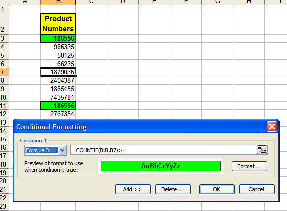 This says, "look through the entire range of column B. Count how many cells in that range are the same value as what is in B3." (In the graphic, B7 is the Active cell.) That same comparison will be made in every cell that contains the conditional formatting. (If your data is in column E and you are setting the first conditional formatting up in E5, the formula would be =COUNTIF(E:E,E5)>1.) Anytime a duplicate appears in the range, it will receive the special formatting. In this example, any time a duplicate number appears anywhere in column B, even if it is not itself formatted, the selected range will reflect the duplicate. =COUNT(B:B,B3)>2 would count entries that appear more than two times. =COUNT(B:B,B3)=2 would count entries that appear twice. If you want only a part of the column in the formula, it is easier to use absolute addresses, such as =COUNT($B$3:$B$200,B3)>1 Adapted from MrExcel.com Also see: Chip Pearson's discussion of duplicates: Duplicate And Unique Items In Lists and: Contextures.com: Conditional Formatting (See Hide Duplicate Values) See all Topics excel Labels: Formulas, General, Macros, Reference, Tips, Tutorials, VBA <Doug Klippert@ 3:11 AM
Comments:
Post a Comment
Wednesday, July 22, 2015 – Permalink – Statistics and ExcelWhat are the chances"Excel is the widely used statistical package, which serves as a tool to understand statistical concepts and computation to check your hand-worked calculation in solving your homework problems. The site provides an introduction to understand the basics of and working with the Excel. Redoing the illustrated numerical examples in this site will help improving your familiarity and as a result increase the effectiveness and efficiency of your process in statistics." Dr. Hossein Arsham The site is very clearly written. While some of the concepts are advanced, Dr. Arsham explains them in simple terms. It is a good introduction to the Analysis ToolPak. Here are some of the subjects covered:
See all Topics excel Labels: Formulas, Functions, General, Reference, Tips, Tutorials <Doug Klippert@ 3:11 AM
Comments:
Post a Comment
|
